Handling the Unseen: Censored Distributions, Measure Theory, and Entropy

In machine learning, we usually assume that our data is observed exactly. The real instruments have intrinsic limits.When the measurement falls beyond a detection limit, it may be reported at the threshold, rather than at its actual value, returning thus a data point that is censored. Such report is not a missing observation: it tells us that the underlying response lies in a particular tail. This is a structural feature of many scientific pipelines, not just an accidental occasion.

Censoring quietly breaks standard regression models, and addressing it properly requires a small excursion into the measure theory.

This is the first post in a short series. We will describe the Tobit observation law, derive its entropy relative to an explicit reference measure, and explain which KL divergences are meaningful. These distinctions matter when turning censored Gaussian models into information-theoretic acquisition functions.

Motivation: Censoring is structural, not anomalous

Most measurements come from instruments with bounded scales. In drug discovery, for example, a high-throughput binding assay cannot resolve affinities beyond its detection limit: it clips non-binders at a threshold $l$, so all we know about such a point is that its true value satisfies $y^\ast \ge l$. The measurement is not missing; it is present, but only as an inequality.

Faced with this, two common shortcuts both introduce bias:

• Drop the censored points. Training a regressor only on the fully-resolved values truncates the distribution. This discards the information that non-binders provide ($y^\ast \ge l$) and degrades uncertainty right at the decision boundary, where it is most important.
• Clamp and pretend. Treating each clipped value as if it were an exact observation and fitting a Gaussian likelihood (or equivalently, minimizing MSE) biases the fit regardless of model architecture; the loss is simply incorrect for those points.

The alternative is to model the recording mechanism. In what follows, “censoring” means deterministic clipping of a noisy real-valued response. It is different from truncation, where observations outside a window are omitted and the retained law must be renormalized.

The Tobit likelihood

Let $f$ be the latent function we want to recover:

Let each observation carry an indicator $c_i \in {-1, 0, 1}$ recording whether it is left-censored, uncensored, or right-censored. With per-point bounds $l_i, u_i$ and noise $\varepsilon \sim \mathcal{N}(0,\sigma^2)$, the observation process is

If we write $\phi$ and $\Phi$ for the standard normal PDF and CDF, and $f_i = f(\mathbf{x}_i)$, the resulting likelihood is a continuous density in the interior and a probit atom at each bound:

We write $L_i(f_i)$, rather than conditioning the probability law on the realized indicator: conditional on being uncensored, the response would have a normalized truncated Gaussian law. The tail probabilities above account for the probability of observing the censoring event itself. The inequality in a censored report concerns $Z_i$, the noisy response. It is not a deterministic inequality on $f(x_i)$ when $\sigma>0$.

This setup matches the physics of the instrument closely, but it creates a mathematical issue.

A distribution that is neither continuous nor discrete

Fix a mean $\mu$, a positive standard deviation $\sigma$, and finite bounds $l<u$. Define

If $G_{\mu,\sigma}=N(\mu,\sigma^2)$, the recorded law is its pushforward under clipping:

As a measure, it is

The continuous part has total mass $p_0$, not one. There is no truncation renormalization: the remaining probability has been moved to the endpoints.

A Dirac measure $\delta_c$ assigns mass one to a measurable set containing $c$, and zero otherwise. Each atom’s weight is exactly the Gaussian tail probability that is collapsed onto the boundary. It is not an ordinary density function that can be substituted into logarithms.

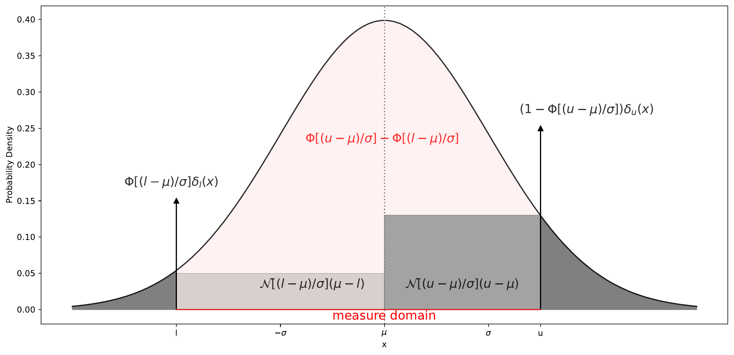The Censored Normal distribution as a mixed measure. The window $(l,u)$ carries the interior mass $\Phi(\tfrac{u-\mu}{\sigma})-\Phi(\tfrac{l-\mu}{\sigma})$ (red), while the two arrows are the boundary atoms with weights $\Phi(\tfrac{l-\mu}{\sigma})$ and $1-\Phi(\tfrac{u-\mu}{\sigma})$ — the collapsed lower and upper tails. The red baseline marks the “measure domain,” the support of the reference measure $\rho=\lambda+\delta_l+\delta_u$.

The measure-theoretic fix

The law cannot have a density with respect to Lebesgue measure alone: a singleton has Lebesgue measure zero, but an endpoint has positive probability.

Choose instead

This reference measure contains both the continuous observation window and the endpoint atoms. Its support is $[l,u]$. The Radon–Nikodym derivative is the ordinary measurable function:

The distinction is important: the measure is written with Dirac measures; its density relative to $\rho$ is written with ordinary values or indicator functions.

Lebesgue decomposition describes the absolutely continuous interior and the singular atomic part relative to Lebesgue measure. The Radon–Nikodym theorem then supplies the density relative to the chosen dominating measure. These are complementary statements, not a replacement for the usual definition of expectation.

For any integrable function $g$,

The law $\nu$ should not be confused with the empirical measure of a finite sample. An empirical measure also has atoms at the observed interior values, so it is generally not dominated by this same $\rho$.

Warm-up: integrating against the mixed measure

Taking $g(y)=y$ gives

The atom terms are simply each boundary value weighted by its collapsed tail probability. For bounds symmetric about $\mu$, the mean remains $\mu$. Notice that the correction $-\sigma[\phi(a)-\phi(b)]$ vanishes when the bounds are symmetric about the mean ($a=-b$): symmetry cancels the interior first-moment correction because $\phi(-d)=\phi(d)$. The analogous second-moment correction in the entropy does not cancel.

Closed-form entropy of the Censored Normal

Carrying the same decomposition through the entropy integral gives a fully closed-form result — no Monte Carlo needed. With $\zeta_x = \tfrac{x-\mu}{\sigma}$ and window mass $\Delta\Phi = \Phi(\zeta_u)-\Phi(\zeta_\ell)$: Define entropy relative to the specified reference measure by

using natural logarithms and $0\log0=0$. For the censored normal above, the integral is finite and evaluates to

The three pieces have clear interpretations:

• Base entropy. $p_0\log!\big(\sqrt{2\pi e}\,\sigma\big)$ is the ordinary Gaussian differential entropy, scaled down by $p_0$, the probability mass that actually falls inside the observable window.
• Boundary (second-moment) correction. $-\frac12[b\phi(b)-a\phi(a)]$ accounts for how clipping changes the spread of the interior; it is the truncated-variance correction to the differential-entropy term. Unlike the mean’s correction above, this one does not vanish for symmetric bounds: there $\zeta_u\phi(\zeta_u)-\zeta_\ell\phi(\zeta_\ell)=2\tfrac{\Delta}{\sigma}\phi(\tfrac{\Delta}{\sigma})$, leaving $-\tfrac{\Delta}{\sigma}\phi(\tfrac{\Delta}{\sigma})$.
• Atom entropy. $-p_l\log p_l-p_u\log p_u$ is the Shannon entropy of the two collapsed tails, each treated as a discrete outcome with its tail probability. Their weights do not themselves sum to one unless there is no interior mass.

Sanity check (uncensoring). As $l\to-\infty$ and $u\to+\infty$ we have $p_0 \to 1$; both $a\phi(a)$, $b\phi(b)$ terms vanish; and since $t\log t\to 0$ as $t\to 1$, the atom terms vanish as well. What remains is

which is exactly the entropy of the underlying Gaussian — the formula smoothly reduces to the familiar case.

An alternative decomposition makes the role of the censoring indicator explicit:

where $H(C)$ is the entropy of the three-outcome probability vector $(p_l,p_0,p_u)$, and $h(Y\mid C=0)$ is the differential entropy of the normalized truncated normal.

Symmetric bounds. For $l=\mu-\Delta$, $u=\mu+\Delta$, with $\Delta>0$, let $d=\Delta/\sigma$ and $q=\Phi(-d)$. Both endpoint probabilities equal $q$. Therefore

The boundary correction is $-d\phi(d)$, not zero. As $\Delta\to\infty$, the ordinary Gaussian entropy is recovered.

Plotting the three terms as the censored fraction increases makes the trade-off clear:

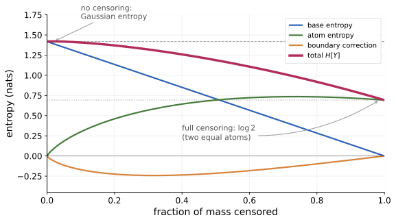The three terms of $H_\rho(Y)$ as more mass is censored (standard normal, symmetric bounds). The base entropy (blue) fades as the observable window shrinks; the atom entropy (green) grows as probability accumulates at the boundaries; the boundary correction (orange) stays negative. Their sum (pink) interpolates smoothly between the Gaussian entropy $\log\sqrt{2\pi e}\,\sigma$ with no censoring and $\log 2$ — two equally likely atoms — under full censoring.

This is a useful way to see how much entropy is removed by clipping as the window narrows.

Why the reference measure matters

If the reference is changed to $d\rho’=w\,d\rho$, with $w>0$, then, when the expectations exist,

Consequently this entropy is not a coordinate-free amount of information lost by clipping. It can also be negative. KL divergence and mutual information, rather than differences between arbitrarily chosen entropies, provide the invariant comparisons.

Which KL divergence is meaningful?

For probability measures $P,Q$,

When both have densities $p,q$ relative to a common reference, this becomes $\int p\log(p/q)\,d\rho$, with value $+\infty$ if the set where $q=0$ has positive $P$-probability. A common dominating measure does not ensure a finite KL.

For an uncensored nondegenerate Gaussian $G$ and a Gaussian law $\nu$ clipped at at least one finite endpoint,

The first direction fails because the Gaussian assigns probability beyond the observation window. The second fails because the censored law has endpoint atoms while the Gaussian assigns zero probability to every singleton.

To compare two latent models through the same instrument, compare their two censored observation laws. If $P=T_#G_1$, $Q=T_#G_0$, with the same bounds, then

where $g_j$ is the uncensored Gaussian density in the interior. No logarithms or ratios of Dirac measures are involved.

Data processing gives a useful check:

Clipping cannot increase the ability to distinguish the two latent models from the observation.

Why this matters

A closed-form, differentiable entropy is the key that enables information-theoretic acquisition under censoring. Once we can evaluate $H[Y]$ exactly, we can build analytic versions of BALD (Bayesian Active Learning by Disagreement) and Predictive Entropy Search that account for the atoms instead of being misled by them. The practical result: instead of models becoming overconfident at detection limits, they can deliberately probe those boundaries, enabling efficient active learning and Bayesian optimization that thrive on censored data instead of failing on it.

That construction — turning this entropy into acquisition functions with consistency and $D$-optimality guarantees — is the subject of the next post in the series.

References

• A. Karlová, R. Kabra, D. A. de Souza, B. Paige. COBALT: Censored Optimization and Bayesian Active Learning Techniques. Proceedings of the 42nd Conference on Uncertainty in Artificial Intelligence (UAI), PMLR 337:2713–2743, 2026. proceedings · PDF · OpenReview

• Yury Polyanskiy and Yihong Wu. Information Theory, MIT 6.441 course notes: divergence, mutual information, data processing, and variational characterizations. Course notes.

• Code: github.com/AndreaKarlova/cobalt

@InProceedings{pmlr-v337-karlova26a,
  title     = { {COBALT}: Censored Optimization and {Bayesian} Active Learning Techniques},
  author    = {Karlova, Andrea and Kabra, Rishabh and de Souza, Daniel Augusto and Paige, Brooks},
  booktitle = {Proceedings of the 42nd Conference on Uncertainty in Artificial Intelligence},
  pages     = {2713--2743},
  year      = {2026},
  editor    = {Perkovi{\'c}, Emilija and Malinsky, Daniel},
  volume    = {337},
  series    = {Proceedings of Machine Learning Research},
  month     = {17--21 Aug},
  publisher = {PMLR},
  url       = {https://proceedings.mlr.press/v337/karlova26a.html}
}